Pseudoholomorphic curves
m (→Moduli spaces) |
(→References) |
||
| Line 100: | Line 100: | ||
== References == | == References == | ||
{{#RefList:}} | {{#RefList:}} | ||
| − | |||
[[Category:Theory]] | [[Category:Theory]] | ||
Latest revision as of 15:56, 20 February 2012
|
This page has not been refereed. The information given here might be incomplete or provisional. |
Contents |
1 Introduction
In this article,  will denote an almost complex manifold of dimension
  .
.
Definition 1.1 ( -holomorphic curve).
Let
-holomorphic curve).
Let  be a Riemann surface with complex structure
  . A
. A  -holomorphic curve

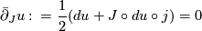
is a smooth map satisfying
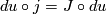
or equivalently
A -holomorphic map is called simple if it cannot be factored as  where
where  is a
is a  -holomorphic branched cover
  of degree strictly greater than 1. We will usually omit from the notation and speak of -holomorphic curves. The term pseudoholomorphic curve will be used to describe a -holomorphic curve when we do not want to specify .
Pseudoholomorphic curves provide a useful tool for studying symplectic manifolds.
2 Taming J
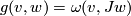
Pseudoholomorphic curves in a general almost complex manifold can be quite wild (EXAMPLE?). Better behaviour can be ensured by the existence of a symplectic  taming , that is the quadratic form
is positive-definite. This gives us topological control on the energy of a -holomorphic curve
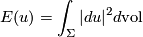
(here the norm and volume form are taken with respect to the metric  ) thanks to the identity
Lemma 2.1 (Energy identity).
If  is a -holomorphic curve and is tamed by then
If moreover we require the metric to be -invariant ( ) then we say that is -compatible and we have the identity
so that the -holomorphic curves are the absolute minima of the energy functional on the space of maps  .
.
3 Linearisation
 as a section of a Banach bundle. Explicitly, let
  denote the
  -completion of the space of maps
  and let
  denote the space of -compatible almost complex structures. Define the Banach bundle
  over
over  whose fibre over
  is the
  -completion of the space
 -forms on
  with values in
  . Here refers to the complex structures on
  and on . By definition,
 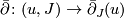 is a section of this bundle over the smooth locus and it extends naturally to the Sobolev completions.
  at a -holomorphic curve is the operator
 on ) by
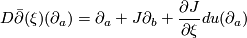
Here we think of as a section of  and
and  as a map
  so
so  means the pushforward of
  along . The linearisation measures to first order the change in
  when is deformed along a vector field . One can also allow to vary in the space of complex structures on or to vary in a family of almost complex structures by adding corresponding terms to the linearisation.
Theorem 3.2 Ellipticity. The linearised Cauchy-Riemann operator of a holomorphic curve is a Fredholm operator.
In the case when is an integrable complex structure the kernel and cokernel of the linearised Cauchy-Riemann operator agree with the usual Dolbeault cohomology groups.
4 Moduli spaces
Simple -holomorphic curves form nice moduli spaces
Theorem 4.1 Transversality for simple curves.
Fix a homology class  and a Riemann surface . There is a subset
  of the second-category such that the space

is a finite-dimensional manifold of dimension
![\displaystyle n(2-2g)+2c_1(X,J)[A]](/images/math/1/e/a/1eaaedc1211195624b75d18a0c41a504.png)
If one allows to vary then this dimension formula gains an extra  if
if  or
or  if
if  .
.
These almost complex structures are the regular almost complex structures, for which the linearised problem has vanishing cokernel. Transversality is achieved by making small perturbations of the almost complex structure in regions through which the pseudoholomorphic curve has to pass.
Usually one defines a moduli space by dividing out the space of parametrised maps by the group of holomorphic reparametrisations. This group is:
-
 , the 6-dimensional group of M\"{o}bius transformations when
  ,
,
-
 , acting by translations when ,
- finite when
Definition 4.2 Expected dimension. The expected dimension of the moduli space is the number
![\displaystyle n(2-2g)+2c_1(X,J)[A]+6g-6](/images/math/6/3/d/63d76165355535a5651d2ed3570fc8c8.png)
and this coincides with the actual dimension of a regular moduli space of curves after dividing out by reparametrisation.
It is harder to achieve transversality for curves which are multiple covers. This is best seen in a simple example.
Example 4.3 Isolated spheres in Calabi-Yau 3-folds.
Consider  , the total space of the bundle
  over
over  . The inclusion of the zero-section
  is the only closed holomorphic curve in its homology class (up to reparametrisation). This sphere is regular; the expected dimension is zero since
  . If
. If  is a generic holomorphic branched cover of degree
  then
then  lives in a moduli space of dimension
  (corresponding to the configuration space of the
  branch points). The expected dimension is still zero, so the linearised operator must have a nontrivial cokernel.
In this case one needs to introduce more general perturbations to achieve transversality.
Theorem 4.4 Transversality in the semipositive case.
When  is semipositive one can achieve transversality even for multiply-covered curves by using a domain-dependent .
5 Compactness
While the  -control on the derivatives of given by the energy identity 2.1 is not enough to ensure a priori compactness of moduli spaces, there is a natural compactification by adding in strata of stable maps.
Definition 5.1 (Stable map).
Let be a nodal Riemann surface (i.e. a connected, compact reduced complex curve with at worst ordinary double points) and  a collection of distinct non-nodal marked points on . A stable map
  is a -holomorphic map such that any irreducible component of which is mapped down to a point
  has either
- arithmetic genus 0 and at least three points which are either marked or nodal,
- arithmetic genus 1 and at least one point which is either marked or nodal,
- arithmetic genus 2 or more.
This is equivalent to the requirement that the group of holomorphic automorphisms of fixing the marked points and satisfying  is finite. A reparametrisation of a stable map is a holomorphic automorphism of the domain which does not necessarily leave invariant and we usually only consider stable maps up to reparametrisation.
There is a notion of convergence for stable maps up to reparametrisation, called Gromov convergence, which allows us to define a topology of the moduli space of stable maps.
Theorem 5.2 (Gromov compactness). The moduli space of stable maps (modulo reparametrisations) with the topology of Gromov convergence is both compact and Hausdorff.