Links of singular points of complex hypersurfaces
| Line 1: | Line 1: | ||
| − | |||
| − | |||
| − | |||
| − | |||
| − | |||
| − | |||
| − | |||
| − | |||
| − | |||
| − | |||
| − | |||
| − | |||
== Introduction == | == Introduction == | ||
| − | <wikitex> | + | <wikitex>; |
| − | The links of singular points of complex hypersurfaces | + | The links of singular points of complex hypersurfaces provide a large class of examples of highly-connected odd dimensional manifolds. A standard reference is {{cite|Milnor1968}}. |
| + | These manifolds are the boundaries of [[highly-connected]], [[stably parallelisable]] even dimensional manifolds and hence stably parallelisable themselves. In the case of singular points of complex curves, the link of such a singular point is a fibered link in the $3$-dimensional sphere $S^3$. | ||
</wikitex> | </wikitex> | ||
| Line 42: | Line 31: | ||
Each fiber is a smooth parallelizable manifold with boundary, having the homotopy type of a bouquet of $n$-spheres $S^n\vee \cdots \vee S^n$. | Each fiber is a smooth parallelizable manifold with boundary, having the homotopy type of a bouquet of $n$-spheres $S^n\vee \cdots \vee S^n$. | ||
\end{thm} | \end{thm} | ||
| − | |||
</wikitex> | </wikitex> | ||
| − | == Invariants | + | == Invariants == |
<wikitex>; | <wikitex>; | ||
Seen from the above section, the link $K$ of an isolated singular point $z$ of a complex hypersurface $V$ of complex dimension $n$ is a $(n-2)$-connected $(2n-1)$-dimensional closed smooth manifold. In high dimensional topology, these are called highly connected manifolds, since for a $(2n-1)$-dimensional closed manifold $M$ which is not a homotopy sphere, $(n-2)$ is the highest connectivity $M$ could have. Therefore to understand the classification and invariants of the links $K$ one needs to understand the classification and invariants of highly-connected odd dimensional manifolds, for which see [[highly-connected_manifolds|highly-connected manifolds]]. | Seen from the above section, the link $K$ of an isolated singular point $z$ of a complex hypersurface $V$ of complex dimension $n$ is a $(n-2)$-connected $(2n-1)$-dimensional closed smooth manifold. In high dimensional topology, these are called highly connected manifolds, since for a $(2n-1)$-dimensional closed manifold $M$ which is not a homotopy sphere, $(n-2)$ is the highest connectivity $M$ could have. Therefore to understand the classification and invariants of the links $K$ one needs to understand the classification and invariants of highly-connected odd dimensional manifolds, for which see [[highly-connected_manifolds|highly-connected manifolds]]. | ||
| Line 54: | Line 42: | ||
</wikitex> | </wikitex> | ||
| − | == Classification | + | == Classification == |
<wikitex>; | <wikitex>; | ||
... | ... | ||
| Line 66: | Line 54: | ||
== References == | == References == | ||
{{#RefList:}} | {{#RefList:}} | ||
| − | |||
| − | |||
[[Category:Manifolds]] | [[Category:Manifolds]] | ||
{{Stub}} | {{Stub}} | ||
Revision as of 17:14, 7 June 2010
Contents |
1 Introduction
The links of singular points of complex hypersurfaces provide a large class of examples of highly-connected odd dimensional manifolds. A standard reference is [Milnor1968].
These manifolds are the boundaries of highly-connected, stably parallelisable even dimensional manifolds and hence stably parallelisable themselves. In the case of singular points of complex curves, the link of such a singular point is a fibered link in the  -dimensional sphere
  .
.
2 Construction and examples
Let 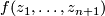 be a non-constant polynomial in
  complex variables. A complex hypersurface
  is the algebraic set consisting of points
 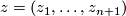 such that
  . A regular point
  is a point at which some partial derivative
  does not vanish; if at a point all the partial derivatives
  vanish,
  is called a singular point of .
Near a regular point , the complex hypersurface is a smooth manifold of real dimension  ; in a small neighborhood of a singular point , the topology of the complex hypersurface is more complicated. One way to look at the topology near , due to Brauner, is to look at the intersection of with a
  -dimensioanl sphere of small radius
 centered at .
\begin{thm}
The space  is
is  -connected.
\end{thm}
-connected.
\end{thm}
The topology of  is independent of the small paremeter , it is called the link of the singular point .
\begin{thm}(Fibration Theorem)
For sufficiently small, the space  is a smooth fiber bundle over
  , with projection map
 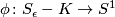 ,
,  . Each fiber
  is parallelizable and has the homotopy type of a finite CW-complex of dimension
  .
\end{thm}
.
\end{thm}
The fiber is usually called the Milnor fiber of the singular point .
A singular point is isolated if there is no other singular point in some small neighborhood of .
In this special situation, the above theorems are strengthened to the following
\begin{thm}
Each fiber is a smooth parallelizable manifold with boundary, having the homotopy type of a bouquet of -spheres  .
\end{thm}
.
\end{thm}
3 Invariants
Seen from the above section, the link of an isolated singular point of a complex hypersurface of complex dimension is a -connected  -dimensional closed smooth manifold. In high dimensional topology, these are called highly connected manifolds, since for a -dimensional closed manifold
  which is not a homotopy sphere, is the highest connectivity could have. Therefore to understand the classification and invariants of the links one needs to understand the classification and invariants of highly-connected odd dimensional manifolds, for which see highly-connected manifolds.
On the other hand, as the link is closely related to the singular point of the complex hypersurfaces, some of the topological invariants of are computable from the polynomial.
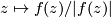
Let be a complex hypersurface defined by ,  be an isolated singular point of . Let
 . By putting all these
  's together we get the gradient field of
  , which can be viewed as a map
  ,
,  .
.
4 Classification
...
5 Further discussion
...
6 References
- [Milnor1968] J. Milnor, Singular points of complex hypersurfaces, Princeton University Press, Princeton, N.J., 1968. MR0239612 (39 #969) Zbl 0224.57014
|
This page has not been refereed. The information given here might be incomplete or provisional. |
.
2 Construction and examples
Let be a non-constant polynomial in complex variables. A complex hypersurface is the algebraic set consisting of points such that . A regular point is a point at which some partial derivative does not vanish; if at a point all the partial derivatives vanish, is called a singular point of .
Near a regular point , the complex hypersurface is a smooth manifold of real dimension ; in a small neighborhood of a singular point , the topology of the complex hypersurface is more complicated. One way to look at the topology near , due to Brauner, is to look at the intersection of with a -dimensioanl sphere of small radius centered at .
\begin{thm}
The space is -connected.
\end{thm}
The topology of is independent of the small paremeter , it is called the link of the singular point .
\begin{thm}(Fibration Theorem)
For sufficiently small, the space is a smooth fiber bundle over , with projection map , . Each fiber is parallelizable and has the homotopy type of a finite CW-complex of dimension .
\end{thm}
The fiber is usually called the Milnor fiber of the singular point .
A singular point is isolated if there is no other singular point in some small neighborhood of .
In this special situation, the above theorems are strengthened to the following
\begin{thm}
Each fiber is a smooth parallelizable manifold with boundary, having the homotopy type of a bouquet of -spheres .
\end{thm}
3 Invariants
Seen from the above section, the link of an isolated singular point of a complex hypersurface of complex dimension is a -connected -dimensional closed smooth manifold. In high dimensional topology, these are called highly connected manifolds, since for a -dimensional closed manifold which is not a homotopy sphere, is the highest connectivity could have. Therefore to understand the classification and invariants of the links one needs to understand the classification and invariants of highly-connected odd dimensional manifolds, for which see highly-connected manifolds.
On the other hand, as the link is closely related to the singular point of the complex hypersurfaces, some of the topological invariants of are computable from the polynomial.
Let be a complex hypersurface defined by , be an isolated singular point of . Let . By putting all these 's together we get the gradient field of , which can be viewed as a map , .
4 Classification
...
5 Further discussion
...
6 References
- [Milnor1968] J. Milnor, Singular points of complex hypersurfaces, Princeton University Press, Princeton, N.J., 1968. MR0239612 (39 #969) Zbl 0224.57014
|
This page has not been refereed. The information given here might be incomplete or provisional. |