High codimension links
| This page has been accepted for publication in the Bulletin of the Manifold Atlas. |
|
The user responsible for this page is Askopenkov. No other user may edit this page at present. |
1 Introduction
Most of this page is intended not only for specialists in embeddings, but also for mathematician from other areas who want to apply or to learn the theory of embeddings.
On this page we describe readily calculable classifications of embeddings of closed disconnected manifolds into  up to isotopy, and more generally of spaces which are a disjoint union of manifolds of varying dimensions. The presently known cases of such classifications are embeddings
  , where
  are spheres (or even closed manifolds) and
  for every
  , under some further restrictions. For a related classification of knotted tori see [Skopenkov2016k].
For an  -tuple
  denote
  . Although
  is not a manifold when
  are not all equal, embeddings
  and isotopy between such embeddings are defined analogously to the case of manifolds [Skopenkov2016i]. Denote by
  the set of embeddings up to isotopy.
For a general introduction to embeddings as well as the notation and conventions used on this page, we refer to [Skopenkov2016c,  1, 3].
The following table was obtained by Zeeman around 1960 (see the Haefliger-Zeeman Theorem 4.1 below):


A component-wise version of embedded connected sum [Skopenkov2016c, 5] defines a commutative group structure on the set for  [Haefliger1966a, 2.5], [Skopenkov2015, Group Structure Lemma 2.2 and Remark 2.3.a], [Avvakumov2016, 1], [Avvakumov2017, 1.4], see Figure 1.
The standard embedding  is defined by
  . Fix pairwise disjoint
  -discs
  . The standard embedding is defined by taking the union of the compositions of the standard embeddings
  with the fixed inclusions
  .
.
2 Examples
Recall that for any  -manifold
  and
and  , every two embeddings
  are isotopic [Skopenkov2016c, General Position Theorem 2.1], [Skopenkov2006, General Position Theorem 2.1].
The following example shows that the restriction is sharp for non-connected manifolds.
are isotopic [Skopenkov2016c, General Position Theorem 2.1], [Skopenkov2006, General Position Theorem 2.1].
The following example shows that the restriction is sharp for non-connected manifolds.
Example 2.1 (The Hopf Link).
(a) For every positive integer there is an embedding  , which is not isotopic to the standard embedding.

For  the Hopf link is shown in Figure 2. For all the image of the Hopf link is the union of two -spheres which can be described as follows:
- either the spheres are
 and
and  in
in  ;
;
- or they are given as the sets of points in
 satisfying the following equations:

This embedding is distinguished from the standard embedding by the linking number (cf. 3).
(b) For any  there is an embedding
  which is not isotopic to the standard embedding.
Analogously to (a), the image is the union of two spheres which can be described as follows:
- either the spheres are
 and in
  .
.
- or they are given as the points in
 satisfying the following equations:

This embedding is also distinguished from the standard embedding by the linking number (cf. 3).
Definition 2.2 (A link with prescribed linking coefficient). We define the `Zeeman' map


For a map  representing an element of
  let
let
Tex syntax error
Tex syntax error. Let
Tex syntax error.
One can easily check that  is well-defined and is a homomorphism.
3 The linking coefficient
Here we define the linking coefficient and discuss its properties. Fix orientations of the standard spheres and balls.
Definition 3.1 (The linking coefficient). We define a map

Take an embedding  representing an element
 ![[f]\in E^m(S^p\sqcup S^q)](/images/math/9/5/8/958e4adb33de7e2445e035db1cbd05a0.png) .
Take an embedding
.
Take an embedding  such that
  intersects
  transversely at exactly one point with positive sign; see Figure 4.

 and Gauss map
Then the restriction  of
of  to
to  is a homotopy equivalence.
(Indeed, since  , by general position the complement
  is simply-connected.
By Alexander duality,
is simply-connected.
By Alexander duality,  induces isomorphism in homology.
Hence by the Hurewicz and Whitehead theorems is a homotopy equivalence.)
induces isomorphism in homology.
Hence by the Hurewicz and Whitehead theorems is a homotopy equivalence.)
Let  be a homotopy inverse of .
Define
be a homotopy inverse of .
Define
![\displaystyle \lambda[f]=\lambda_{12}[f]:=[S^p\xrightarrow{~f|_{S^p}~} S^m-fS^q\overset h\to S^{m-q-1}]\in\pi_p(S^{m-q-1}).](/images/math/7/0/2/702421c61c119e9f17cfea8b085f374a.png)
Remark 3.2.
(a) Clearly, ![\lambda[f]](/images/math/4/6/0/4603ad5fae840a15ed28fd021825efae.png) is well-defined, i.e. is independent of the choices of
is well-defined, i.e. is independent of the choices of  and of the representative
  of
of ![[f]](/images/math/d/d/4/dd43b82529dd8d403c1585c5d151a163.png) .
One can check that
.
One can check that  is a homomorphism.
(b) Analogously one can define ![\lambda_{21}[f]\in\pi_q(S^{m-p-1})](/images/math/5/b/8/5b81499fd01f4267c2347d2439817f40.png) for
for  , by exchanging
  and in the above definition.
(c) Clearly,  for the Zeeman map . So is surjective and is injective.
(d) For  there is a simpler alternative definition using homological ideas. That definition can be generalized to the case where the components are closed orientable manifolds. Cf. Remark 5.3.f of [Skopenkov2016e].
Recall that by the Freudenthal Suspension Theorem the stable suspension homomorphism  is an isomorphism for
  . The stable suspension of the linking coefficient can be described as follows.
Definition 3.3 (The  -invariant). We define a map
 for
for  .
Take an embedding representing an element .
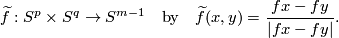
Define the Gauss map (see Figure 4)
.
Take an embedding representing an element .
Define the Gauss map (see Figure 4)
For define the -invariant by
![\displaystyle \alpha[f]=[\widetilde f]\in[S^p\times S^q,S^{m-1}]\overset{v^*}\cong\pi_{p+q}(S^{m-1})\cong\pi^S_{p+q+1-m}.](/images/math/5/3/d/53debfbd4a5d88f0c6d79b4fce1d64a3.png)
The second isomorphism in this formula is the suspension isomorphism.
The map 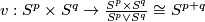 is the quotient map, see Figure 5.

The map  is a 1--1 correspondence for
  .
(For this follows by general position and for
.
(For this follows by general position and for  by the cofibration Barratt-Puppe exact sequence of pair
  and by the existence of a retraction
  .)
.)
One can easily check that is well-defined and for  is a homomorphism.
Lemma 3.4 [Kervaire1959a, Lemma 5.1].
We have  for .
for .
Hence  , even though in general
  as we explain in Example 5.2.a,c.
Note that the -invariant can be defined in more general situations [Koschorke1988], [Skopenkov2006, 5].
4 Classification in the metastable range
The Haefliger-Zeeman Theorem 4.1.
If  , then both and are isomorphisms for
  in the smooth category, and for in the PL category.
The surjectivity of (or the injectivity of ) follows from  .
The injectivity of (or the surjectivity of ) is proved in [Haefliger1962t, Theorem in 5], [Zeeman1962]
(or follows from [Skopenkov2006, the Haefliger-Weber Theorem 5.4 and the Deleted Product Lemma 5.3.a]).
.
The injectivity of (or the surjectivity of ) is proved in [Haefliger1962t, Theorem in 5], [Zeeman1962]
(or follows from [Skopenkov2006, the Haefliger-Weber Theorem 5.4 and the Deleted Product Lemma 5.3.a]).
An analogue of this result holds for links with many components, each of the same dimension [Haefliger1962t, Theorem in 5]. Let  be the -tuple consisting entirely of some positive integer .
Theorem 4.2. The collection of pairwise linking coefficients
is a 1-1 correspondence for .
5 Examples beyond the metastable range
For  the results of this section are parts of low-dimensional link theory, so they were known well before given references.
First we present an example of the non-injectivity of the collection of pairwise linking coefficients, which shows that the dimension restriction is sharp in Theorem 4.2.
Example 5.1 (Borromean rings).
(a) There is a non-trivial embedding  whose restriction to each 2-component sublink is trivial [Haefliger1962, 4.1], [Haefliger1962t, 6].
In order to construct such an embedding, denote coordinates in  by
by  .
The (higher-dimensional) `Borromean spheres' are given by the following three systems of equations:
.
The (higher-dimensional) `Borromean spheres' are given by the following three systems of equations:


See Figure 6. The required embedding, called Borromean link, is any embedding whose image is the union of the Borromean spheres.
(b) By moving two of the Borromean spheres and self-intersecting them, we can drag the remaining sphere far away from the two.
More precisely, each two of the Borromean spheres span two (intersecting)  -disks disjoint from the remaining sphere.
(c) Restriction of the Borromean link to each 2-component sublink is trivial, because each two of the Borromean spheres span two disjoint -disks (intersecting the remaining sphere).
Moreover, we can take these -disks so that
- each one of them intersects the remaining sphere transversely by an
 -sphere;
- the obtained two disjoint -spheres in the remaining sphere have linking number
 , i.e. one of them spans an
  -disk (in the remaining sphere) itersecting the other transversely at exacly one point.
(d) The Borromean link is distinguished from the standard embedding by triple linking number of Milnor-Haefliger-Steer-Massey defined as follows (cf. (c)).
Take a 3-component link, i.e. an embedding  .
Assume that is pairwise unlinked, i.e. every two components are contained in disjoint smooth balls.
Let
.
Assume that is pairwise unlinked, i.e. every two components are contained in disjoint smooth balls.
Let  be disjoint oriented embedded -disks in general position to
  , and such that
  for
for  .
Then for
.
Then for  the preimage
  is an oriented -submanifold of
  missing
  .
Let
.
Let  be the linking number of
  and
and  in .
in .
(e) In a standard way one checks that the triple linking number is well-defined, i.e. is independent of the choice of  , and of the isotopy of .
The above definition is equivalent to the standard definition of Milnor-Haefliger-Steer-Massey number [Haefliger1962t, 4], [HaefligerSteer1965], [Haefliger1966a, proof of Theorem 9.4], [Massey1968], [Massey1990, 7] by the well-known `linking number' definition of the Whitehead invariant
, and of the isotopy of .
The above definition is equivalent to the standard definition of Milnor-Haefliger-Steer-Massey number [Haefliger1962t, 4], [HaefligerSteer1965], [Haefliger1966a, proof of Theorem 9.4], [Massey1968], [Massey1990, 7] by the well-known `linking number' definition of the Whitehead invariant  [Skopenkov2020e, 2, Sketch of a proof of (b1)].
If is pairwise unlinked, then the number
[Skopenkov2020e, 2, Sketch of a proof of (b1)].
If is pairwise unlinked, then the number  is independent of permutation of the components, up to multiplication by [HaefligerSteer1965] (this can be easily proved directly).
(f) The Borromean link is non-trivial also because joining the three components with two tubes (i.e. `linked analogue' of embedded connected sum of the components [Skopenkov2016c, 4]) yields a non-trivial knot [Haefliger1962, Theorem 4.3], cf. the Haefliger Trefoil knot [Skopenkov2016t, Example 2.1].
Next we present an example of the non-injectivity of the linking coefficient, which shows that the dimension restriction is sharp in Theorem 4.1.
Example 5.2 (Whitehead link). (a) For every positive integer there is a non-trivial embedding  such that the second component is null-homotopic in the complement of the first component (i.e. the linking coefficient
  is trivial).


Such an embedding is obtained from the Borromean rings embedding by joining the second and the third components with a tube, i.e. by the `linked analogue' of the embedded connected sum of the components [Skopenkov2016c, 3, 4]; see also the Wikipedia article on the Whitehead link. (For the connected sum is not well-defined, so we take the specific connected sum (w) from Figure 7.)
(b) The second component is null-homotopic in the complement of the first component by Example 5.1.b.
(c) For  the Whitehead link is non-trivial because the first component is not null-homotopic in the complement of the second component.
More precisely,
the Whitehead link is non-trivial because the first component is not null-homotopic in the complement of the second component.
More precisely,  equals to the Whitehead square
 ![[\iota_l,\iota_l]\ne0](/images/math/0/0/1/001153eef02a680fe884d6a411e57806.png) of the generator
of the generator  [Haefliger1962t, end of 6] (I do not know a written proof of this except [Skopenkov2015a, the Whitehead link Lemma 2.14] for even).
For
[Haefliger1962t, end of 6] (I do not know a written proof of this except [Skopenkov2015a, the Whitehead link Lemma 2.14] for even).
For  the Whitehead link is distinguished from the standard embedding by more complicated Sato-Levine invariant [Skopenkov2006a].
(d) This example (in higher dimensions, i.e. for  ) seems to have been discovered by Whitehead, in connection with Whitehead product.
(e) For some results on links  related to the Whitehead link see [Skopenkov2015a, 2.5].
6 Linked manifolds
In this section we state some analogues of Theorem 4.2 where spheres are replaced by general manifolds. We start with a simple case where no high-connectivity assumptions are made on the source manifolds.
Theorem 6.1. Assume that  are closed connected manifolds and
  for every . Then for an embedding
  and every
  one defines the linking coefficient
  , see Remark 3.2.e. We have
  if both
  and
and  are orientable, and
  otherwise. Then the collection of pairwise linking coefficients
is well-defined and is a 1-1 correspondence, where  of are orientable and
  are not.
We present the general case of the classification of embeddings of disjoint highly-connected manifolds only for the case of two oriented components of the same dimension.
Theorem 6.2. Let  and
and  be closed
  -dimensional homologically
  -connected orientable manifolds. For an embedding
  one can define the invariant
  analogously to Definition 3.3. Then

is well-defined and is a 1-1 correspondence, provided  .
.
Theorems 6.1 and 6.2 are easily deduced from the Zeeman/Haefliger Unknotting Theorem in the PL/smooth category [Ivansic&Horvatic1974]. They are also corollaries of [Skopenkov2006, the Haefliger-Weber Theorem 5.4] (in both categories); the calculations are analogous to the construction of the 1-1 correspondence ![[S^p\times S^q,S^{m-1}]\to\pi^S_{p+q+1-m}](/images/math/2/b/0/2b09988667478f4877c99836023893d9.png) in Definition 3.3.
See [Skopenkov2000, Proposition 1.2] for the link map analogue.
in Definition 3.3.
See [Skopenkov2000, Proposition 1.2] for the link map analogue.
Now we present an extension of Theorems 6.1 and 6.2 to a case where  and
and  . In particular, for the results below
  ,
,  and the manifolds are only
  -connected. An embedding
  is Brunnian if its restriction to each component is isotopic to the standard embedding. For each triple of integers
  such that
  is even, Avvakumov has constructed a Brunnian embedding
  , which appears in the next result [Avvakumov2016, 1].
Theorem 6.3. [Avvakumov2016, Theorem 1]
Any Brunnian embedding is isotopic to  for some integers such that is even. Two embeddings and
  are isotopic if and only if
  and both
  and
and  are divisible by
  .
.
The proof uses M. Skopenkov's classification of embeddings  (Theorem 8.1 for
  ). The following corollary shows that the relation between the embeddings and is not trivial.
Corollary 6.4. [Avvakumov2016, Corollary 1], cf. [Skopenkov2016t, Corollary 3.5.b]
There exist embeddings  and
and  such that the componentwise embedded connected sum
  is isotopic to
  but is not isotopic to
  .
.
For an unpublished generalization of Theorem 6.3 and Corollary 6.4 see [Avvakumov2017].
7 Reduction to the case with unknotted components
In this section we assume that  is an -tuple such that
  .
.
Define  to be the subgroup of links all whose components are unknotted, i.e. isotopic to the standard embedding
  . We remark that
  [Haefliger1966a,
  2.4, 2.6 and 9.3], [Crowley&Ferry&Skopenkov2011, 1.5].
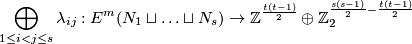
Define the restriction homomorphism by mapping the isotopy class of a link to the ordered -tuple of the isotopy classes of its components:
![\displaystyle r \colon E^m_D(S^{(n)}) \to \bigoplus_{i=1}^s E^m_D(S^{n_i}), \quad r[f]:=\oplus_{i=1}^s [f|_{S^{n_i}} \colon S^{n_i} \to S^m].](/images/math/2/5/d/25d2ec311c8371fe4ac42f34989c9ad0.png)
Take pairwise disjoint -discs in  , i.e. take an embedding
  . Define
![\displaystyle j \colon \bigoplus_{i=1}^s E^m_D(S^{n_i}) \to E^m_D(S^{(n)})\quad\text{by}\quad j([f_1], \ldots, [f_s]):=[(g\circ\sqcup_{i=1}^s f_i):S^{(n)}\to S^m].](/images/math/3/2/9/329c5a3b46fae2defd6d32e45fb15014.png)
Then  is a right inverse of the restriction homomorphism
  , i.e.
  .
The unknotting homomorphism
.
The unknotting homomorphism  is defined to be the homomorphism

Informally, the homomorphism is obtained by taking embedded connected sums of components with knots  representing the elements of
  inverse to the components, whose images
  are small and are close to the components.
For some information on the groups  see [Skopenkov2016s], [Skopenkov2006, 3.3].
8 Classification beyond the metastable range
Theorem 8.1.
[Haefliger1966a, Theorem 10.7], [Skopenkov2009, Theorem 1.1], [Skopenkov2006b, Theorem 1.1]
If  and
and  , then there is a homomorphism
  for which the following map is an isomorphism

The map and its right inverse  are constructed in [Haefliger1966a, 10] and in [Haefliger1966, 8.13], respectively. For alternative geometric (and presumably equivalent) definitions of see [Skopenkov2009, 3], [Skopenkov2006b, 5], cf. [Skopenkov2007, 2] and [Crowley&Skopenkov2016, 2.3]. For a historical remark see [Skopenkov2009, the second paragraph in p. 2].
Remark 8.2.
(a) Theorem 8.1 implies that for any  we have an isomorphism

(b) For any  , the map

is injective and its image is  .
.
For  see [Haefliger1962t, 6]. The following proof for
  and general remark are intended for specialists.
For there is an exact sequence  ,
where
,
where  is
is  [Haefliger1966a, Corollary 10.3].
We have
[Haefliger1966a, Corollary 10.3].
We have  ,
,  and
and  is the reduction modulo 2.
By the exactness of the previous sequence,
is the reduction modulo 2.
By the exactness of the previous sequence,  .
By (a)
.
By (a)  .
Hence
.
Hence  is injective.
We have
is injective.
We have  by [Haefliger1966a, Proposition 10.2].
So the formula of (b) follows.
by [Haefliger1966a, Proposition 10.2].
So the formula of (b) follows.
Analogously to [Skopenkov2009, Theorem 3.5] using geometric definitons of [Skopenkov2009, 3], [Skopenkov2006b, 5] and geomeric interpretation of the EHP sequence  [Koschorke&Sanderson1977, Main Theorem in 1] one can possibly prove that
  . Then (b) would follow.
(c) For any  the map
  in (b) above is not injective [Haefliger1962t, 6].
Theorem 8.3.
For any  there an isomorphism

which is the sum of 3 pairwise invariants of Remark 8.2.a, and the triple linking number (5).
This follows from [Haefliger1966a, Theorem 9.4], see also [Haefliger1962t, 6].
9 Classification in codimension at least 3
In this section we assume that is an -tuple such that .
For this case a readily calculable classification of  was obtained in
[Crowley&Ferry&Skopenkov2011, Theorem 1.9]. In particular, [Crowley&Ferry&Skopenkov2011, 1.2] contains necessary and sufficient conditions on which determine when
was obtained in
[Crowley&Ferry&Skopenkov2011, Theorem 1.9]. In particular, [Crowley&Ferry&Skopenkov2011, 1.2] contains necessary and sufficient conditions on which determine when  is finite. These results are elementary, but the precise formulations are technical. Hence, we only state the following corollary of [Crowley&Ferry&Skopenkov2011, Theorem 1.9 and 1.2] and describe the methods of its proof in Definition 9.2 and Theorem 9.3 below.
Theorem 9.1. There are algorithms which for integers 
Tex syntax error.
(b) determine whether is finite.
Definition 9.2 (The Haefliger link sequence). In [Haefliger1966a, 1.2-1.5] Haefliger defined a long exact sequence of abelian groups

We briefly define the groups and homomorphisms in this sequence, refering to [Haefliger1966a, 1.4] for details.
We first note that in the sequence above the -tuples  are the same for different terms.
Denote
are the same for different terms.
Denote  .
For any
.
For any  and positive integer
  denote by
  the homomorphism induced by the collapse map onto to the -component of the wedge. Denote
  and
and  .
.
It can be shown that each component of a link  has a non-zero normal vector field. So each component of a link can be pushed off along such a vector field into the complement
  . Analogously to Definition 3.1 there is a canonical homotopy equivalence
  . It can also be shown that the homotopy class in of the push off of the th component gives a well-defined map
  . In fact, the map
  is a generalization of the linking coefficient. Finally, define
  .
.
Taking the Whitehead product with the class of the inclusion of  into
into  defines a homomorphism
  . Define
  .
.
The definition of the homomorphism is given in [Haefliger1966a, 1.5].
Theorem 9.3. (a) [Haefliger1966a, Theorem 1.3] The Haefliger link sequence is exact.
(b) The map  is an isomorphism.
Part (b) follows because  [Crowley&Ferry&Skopenkov2011, Lemma 1.3], and so the Haefliger link sequence after tensoring with the rational numbers
  splits into short exact sequences.
In general, the computation of the groups and homomorphisms appearing in Theorem 9.3 is difficult. For (a) no computations are known except for those giving (b) and those giving Theorem 8.1 for  (note that Theorem 8.1 has a direct proof easier than proof of Theorem 9.3.a). For (b) the computations constitute most of [Crowley&Ferry&Skopenkov2011]. Hence Theorem 9.3 is not a readily calculable classification in general.
10 References
- [Avvakumov2016] S. Avvakumov, The classification of certain linked 3-manifolds in 6-space, Moscow Mathematical Journal, 16:1 (2016) 1-25. http://arxiv.org/abs/1408.3918.
- [Avvakumov2017] S. Avvakumov, The classification of linked 3-manifolds in 6-space, Algebraic & Geometric Topology, to appear. arxiv preprint.
- [Crowley&Ferry&Skopenkov2011] D. Crowley, S.C. Ferry, M. Skopenkov, The rational classification of links of codimension >2, Forum Math. 26 (2014), 239-269. https://arxiv.org/abs/1106.1455
- [Crowley&Skopenkov2016] D. Crowley and A. Skopenkov, Embeddings of non-simply-connected 4-manifolds in 7-space, I. Classification modulo knots, Moscow Math. J., 21 (2021), 43--98. arXiv:1611.04738.
- [Haefliger1962] A. Haefliger, Knotted
 -spheres in
  -space, Ann. of Math. (2) 75 (1962), 452–466. MR0145539 (26 #3070) Zbl 0105.17407
- [Haefliger1962t] A. Haefliger, Differentiable links, Topology, 1 (1962) 241--244
- [Haefliger1966] A. Haefliger, Differential embeddings of
 in
in  for
for  , Ann. of Math. (2) 83 (1966), 402–436. MR0202151 (34 #2024) Zbl 0151.32502
- [Haefliger1966a] A. Haefliger, Enlacements de sphères en co-dimension supérieure à 2, Comment. Math. Helv.41 (1966), 51-72. MR0212818 (35 #3683) Zbl 0149.20801
- [HaefligerSteer1965] A. Haefliger and B. Steer, Symmetry of linking coefficients, Comment. Math. Helv., 39 (1965), 259--270.pdf
- [Ivansic&Horvatic1974] I. Ivan\v{s}i\'c and K. Horvati\'c, On unlinking of polyhedra, Glasnik Mat. 9(29) (1974) 147-153.
- [Kervaire1959a] M. Kervaire, An interpretation of G. Whitehead's generalization of H. Hopf's invariant, Ann. of Math. 62 (1959) 345--362.
- [Koschorke&Sanderson1977] U. Koschorke and B. Sanderson, Geometric interpretation of the generalized Hopf invariant, Math. Scand. 41 (1977) 199--217.
- [Koschorke1988] U. Koschorke, Link maps and the geometry of their invariants, Manuscripta Math. 61:4 (1988) 383--415.
- [Massey1968] W. S. Massey, Higher order linking numbers, Proc. Conf. on Algebraic Topology, Univ. Illinois, Chicago Circle, Chicago, Ill., (1968) pp. 174--205. MR0254832 (40 #8039), see also MR1625365 (99e:57016) massey.pdf.
- [Massey1990] W. S. Massey, Homotopy classification of 3-component links of codimension greater than 2, Topol. Appl. 34 (1990) 269--300.
- [Skopenkov2000] A. Skopenkov, On the generalized Massey-Rolfsen invariant for link maps, Fund. Math. 165 (2000), 1-15.
- [Skopenkov2006] A. Skopenkov, Embedding and knotting of manifolds in Euclidean spaces, in: Surveys in Contemporary Mathematics, Ed. N. Young and Y. Choi, London Math. Soc. Lect. Notes, 347 (2008) 248-342. Available at the arXiv:0604045.
- [Skopenkov2006a] A. Skopenkov, Classification of embeddings below the metastable dimension. Available at the arXiv:0607422.
- [Skopenkov2006b] M. Skopenkov, A formula for the group of links in the 2-metastable dimension, arxiv:math/0610320v1
- [Skopenkov2007] A. Skopenkov, A new invariant and parametric connected sum of embeddings, Fund. Math. 197 (2007), 253–269. arXiv:math/0509621. MR2365891 (2008k:57044) Zbl 1145.57019
- [Skopenkov2009] M. Skopenkov, Suspension theorems for links and link maps. Proc. AMS 137 (2009) 359--369. arxiv:math/0610320, version 2 or higher
- [Skopenkov2015] M. Skopenkov, When is the set of embeddings finite up to isotopy? Intern. J. Math. 26:7 (2015), http://arxiv.org/abs/1106.1878
- [Skopenkov2015a] A. Skopenkov, A classification of knotted tori, Proc. A of the Royal Society of Edinburgh, 150:2 (2020), 549-567. Full version: http://arxiv.org/abs/1502.04470
- [Skopenkov2016c] A. Skopenkov, Embeddings in Euclidean space: an introduction to their classification, to appear to Bull. Man. Atl.
- [Skopenkov2016e] A. Skopenkov, Embeddings just below the stable range: classification, to appear in Bull. Man. Atl.
- [Skopenkov2016i] A. Skopenkov, Isotopy, submitted to Bull. Man. Atl.
- [Skopenkov2016k] A. Skopenkov, Knotted tori, preprint.
- [Skopenkov2016s] A. Skopenkov, Knots, i.e. embeddings of spheres, preprint.
- [Skopenkov2016t] A. Skopenkov, 3-manifolds in 6-space, to appear in Boll. Man. Atl.
- [Skopenkov2020e] A. Skopenkov, Extendability of simplicial maps is undecidable, Discr. Comp. Geom., 69:1 (2023), 250–259. arXiv:2008.00492
- [Zeeman1962] E. C. Zeeman, Isotopies and knots in manifolds, Topology of 3-manifolds and related topics (Proc. The Univ. of Georgia Institute, 1961), Prentice-Hall (1962), 187–193. MR0140097 (25 #3520) Zbl 1246.57069