Contact manifold
|
An earlier version of this page was published in the Definitions section of the Bulletin of the Manifold Atlas: screen, print. You may view the version used for publication as of 15:15, 19 November 2013 and the changes since publication. |
|
The user responsible for this page is Hansjörg Geiges. No other user may edit this page at present. |
Contents |
1 Definition
Let  be a differential manifold,
  its tangent bundle, and
  a field of hyperplanes on , that is, a smooth sub-bundle of codimension
  . Here the terms `differential' and `smooth' are used synonymously with
  . Locally,
  can be written as the kernel of a non-vanishing differential -form
  . A -form defined globally on with
  can be found if and only if is coorientable, which is equivalent to saying that the quotient line bundle
  is trivial. The -form is determined by up to multiplication by a smooth function
  or, if the coorientation of has been fixed, by a function taking positive real values only. An equation of the form
  , with a non-vanishing -form, is classically referred to as a Pfaffian equation.
Definition 1.1.
Let be a smooth manifold of odd dimension  . A contact structure on is a hyperplane field whose (locally) defining -form has the property that the
  -form
-form  is nowhere zero, i.e. a volume form, on its domain of definition.
 is indeed a property of and independent of the choice of defining -form , since
Definition 1.2.
A pair  consisting of an odd-dimensional manifold and a contact structure on is called a contact manifold.
Definition 1.3.
A -form as in Definition 1.1, defined globally on , is called a contact form on .
Occasionally the terminology strict contact manifold is used to denote a pair  consisting of an odd-dimensional manifold and a contact form on it.
2 Examples
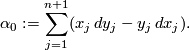
2.1 The standard contact structure on R2n+1
On  with Cartesian coordinates
 -form
-form 
 is called the standard contact structure on . See Figure 1 for the
  -dimensional case.


The theorem of Darboux states that locally any contact structure looks like the standard one, cf. [Geiges2008, Theorem 2.5.1].
Theorem 2.1 (Darboux).
Let be a contact form on the -dimensional manifold and  a point in . Then there are coordinates
  on a neighbourhood
  of such that
  and
and  is given by the contact form
 is equivalent to
  in the following sense.
Definition 2.2.
Two contact manifolds ,  are said to be contactomorphic if there is a diffeomorphism
  with
with  , where
 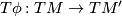 denotes the differential of
  . If
. If  are contact forms defining the contact structures
  , respectively, this is equivalent to saying that and
  determine the same hyperplane field, and hence equivalent to the existence of a nowhere zero function such that
  .
.
where the function  is constant equal to . This is called a strict contactomorphism of the corresponding strict contact manifolds. In the example, the strict contactomorphism
  is given by
 and
and  stand for
  and
and  , respectively, and
  stands for
  .
.
2.2 The standard contact structure on S2n+1
Let  be Cartesian coordinates on
  . Then the standard contact structure
  on the unit sphere
  in is given by the contact form
Write  for the radial coordinate on
  , that is,
 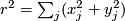 . One checks easily that
 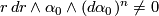 for
for  . Since is a level set of (or
  ), this verifies the contact condition. Alternatively, one may regard as the unit sphere in
  . Then the contact structure may be viewed as the hyperplane field of complex tangencies. Indeed, write
  for the complex structure on corresponding to the complex coordinates
  , that is,
  . Then

which means that defines at each point  the -invariant subspace of
  . Equation (1) follows from the observation that
 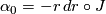 .
.
Here is a further example of contactomorphic manifolds.
Proposition 2.3.
For any point , the contact manifolds  and
and  are contactomorphic.
This is slightly less obvious than it may seem, since stereographic projection does not quite do the job. For a proof of this proposition, due to Erlandsson, see [Geiges2008, Proposition 2.1.8].
2.3 The space of contact elements
Let  be a smooth
  -dimensional manifold. A contact element is a hyperplane in a tangent space to . The space of contact elements of is the collection of pairs
  consisting of a point
  and a contact element
  . This space of contact elements can be naturally identified with the projectivised cotangent bundle
  , by associating with a hyperplane the linear map
  , well defined up to multiplication by a non-zero scalar, with
  . The space is a manifold of dimension
  , and it carries a natural contact structure as defined in the following proposition.
Proposition 2.4.
Write  for the bundle projection
  . For
. For 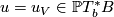 , let
, let  be the hyperplane in
  such that
  is the hyperplane
  in
in  defined by
  . Then defines a contact structure on .
Figure 2 illustrates the construction for  . Here
  .
.

 be local coordinates on , and
  the corresponding dual coordinates in the fibres of the cotangent bundle
  . This means that the coordinate description of covectors is given by
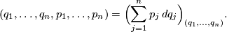
 defines the hyperplane
 , where
 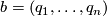 . By construction, the natural contact structure on is defined by
 , although the -form
  is not. In order to verify the contact condition for , we restrict to affine subspaces of the fibre. Over the open set
  , for instance, is defined in terms of affine coordinates
  ,
,  , by the equation
 .
.

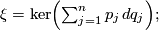
2.4 A non-coorientable contact structure
In the previous example, we now specialise to  . Then the space of contact elements is
  . In terms of Cartesian coordinates
  on
on  and homogeneous coordinates
  on
on  , the natural contact structure on this space of contact elements is now defined globally by equation (2). For
  , and identifying
  with
with  with coordinate
  , this natural contact structure can be written as

This is an example of a contact structure that is not coorientable. It lifts to a coorientable contact structure on  , given by the same equation, with
  . Similar orientability issues arise for general . Write
  and for the natural contact structure on this space of contact elements. We claim the following:
- If is even, then is orientable; is neither orientable nor coorientable.
- If is odd, then is not orientable; is not coorientable, but it is orientable.
The statement about orientability of follows from the corresponding statement for . The fact that is never coorientable follows from the observation that can be identified with the canonical line bundle on (pulled back to ), which is known to be non-trivial, see [Geiges2008, Proposition 2.1.13]. In case (i), since is orientable but not coorientable, it follows that cannot be orientable. The fact that in case (ii) the contact structure is orientable is the consequence of a more general statement in the next section.
2.5 More orientability issues
Notice that a contact manifold with a coorientable contact structure is always orientable (and so is the contact structure), because a globally defined contact form gives rise to a volume form on the manifold. This gives a quicker way to see that in our previous example for odd the contact structure cannot be coorientable. But even for contact structures that need not be coorientable one has the following:
- Any contact manifold of dimension
 is naturally oriented.
 - Any contact structure on a manifold of dimension
 is naturally oriented.
Statement (i) follows from the observation that the sign of the volume form  does not depend on the choice of (local) -form defining the contact structure. Similarly, in case (ii) the sign of
  does not depend on the choice of .
2.6 Three-dimensional contact manifolds
One can easily write down examples of contact structures on some closed -manifolds. The -sphere is dealt with in Section 2.2. The contact structure from equation (3) in Section 2.4 descends to a contact structure on the -torus 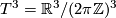 . On
. On 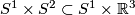 one has the contact structure
 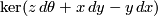 . Notice that by the previous section a -dimensional contact manifold is necessarily orientable. In fact, as shown by Martinet [Martinet1971], this is the only restriction.
Theorem 2.5 [Martinet].
Every closed, orientable -manifold admits a contact structure.
2.7 Brieskorn manifolds
 be an
be an  -tupel of integers
  , and set
  denoting the unit sphere in , we define
  . Manifolds of this form are called Brieskorn manifolds [Brieskorn1966]. It can be shown that the standard contact form on induces a contact structure on
  . This has been observed independently by Abe-Erbacher, Lutz-Meckert and Sasaki-Hsü, cf. [Geiges2008, Section 7.1].
3 A brief history of the terminology
The concept of a contact element first appeared in systematic form in 1896 in the work of Sophus Lie [Lie1896]. His terminology was a little more specific, for instance, a contact element of the plane was called a line element (Linienelement). A contact transformation (Berührungstransformation) for Lie was defined as above, but he only considered this in the context of spaces of contact elements and their natural contact structure (which did not yet bear that name). Such contact transformations play a significant role in the work of E. Cartan, E. Goursat, H. Poincaré and others in the second half of the 19th century. For instance, the Legendre transformation in classical mechanics is a contact transformation. The study of contact manifolds in the modern sense can be traced back to the work of Georges Reeb [Reeb1952], who referred to a strict contact manifold as a `système dynamique avec invariant intégral de Monsieur Elie Cartan'. The relation with dynamical systems comes from the fact that a contact form gives rise to a vector field  defined uniquely by the equations

This vector field is nowadays called the Reeb vector field of . The words `contact structure' and `contact manifold' seem to make their first appearance in the work of Boothby-Wang [Boothby&Wang1958], Gray [Gray1959] and Kobayashi [Kobayashi1959] in the late 1950s. For more historical information on contact manifolds see [Lutz1988] and [Geiges2001].
4 References
- [Boothby&Wang1958] W. M. Boothby and H. C. Wang, On contact manifolds, Ann. of Math. (2) 68 (1958), 721–734. MR0112160 (22 #3015) Zbl 0084.39204
- [Brieskorn1966] E. Brieskorn, Beispiele zur Differentialtopologie von Singularitäten, Invent. Math. 2 (1966), 1–14. MR0206972 (34 #6788) Zbl 0145.17804
- [Geiges2001] H. Geiges, A brief history of contact geometry and topology, Expo. Math. 19 (2001), 25–53. MR1820126 (2002c:53129) Zbl 1048.53001
- [Geiges2008] H. Geiges, An introduction to contact topology, Cambridge Stud. Adv. Math. 109, Cambridge University Press, 2008. MR2397738 (2008m:57064) Zbl 1153.53002
- [Gray1959] J. W. Gray, Some global properties of contact structures, Ann. of Math. (2) 69 (1959), 421–450. MR0112161 (22 #3016) Zbl 0092.39301
- [Kobayashi1959] S. Kobayashi, Remarks on complex contact manifolds, Proc. Amer. Math. Soc. 10 (1959), 164–167. MR0111061 (22 #1925) Zbl 0090.38502
- [Lie1896] S. Lie, Geometrie der Berührungstransformationen (dargestellt von S. Lie und G. Scheffers), B. G. Teubner, Leipzig, 1896. MR0460049 (57 #45) Zbl 03630675
- [Lutz1988] R. Lutz, Quelques remarques historiques et prospectives sur la géométrie de contact, in: Conference on Differential Geometry and Topology, (Sardinia, 1988) Rend. Sem. Fac. Sci. Univ. Cagliari 58 (1988), no.suppl., 361–393. MR1122864 (93b:53025)
- [Martinet1971] J. Martinet, Formes de contact sur les variétés de dimension , Proc. Liverpool Singularities Sympos. II, Lecture Notes in Math. 209, Springer-Verlag, Berlin (1971), 142–163. MR0350771 (50 #3263) Zbl 0215.23003
- [Reeb1952] G. Reeb, Sur certaines propriétés topologiques des trajectoires des systèmes dynamiques, Acad. Roy. Belgique. Cl. Sci. Mém. Coll. in 8
 27, no.9 (1952). MR0058202 (15,336b) Zbl 0048.32903
5 External links
- The Encyclopedia of Mathematics article on contact structure
- The Wikipedia page about contact geometry