6-manifolds: 1-connected

The user responsible for this page is Alexey Zhubr. No other user may edit this page at present.

1 Introduction

Let $\mathcal{M}_6^\Cat$$\newcommand{\Z}{\mathbb{Z}} \newcommand{\R}{\mathbb{R}} \newcommand{\C}{\mathbb{C}} \newcommand{\N}{\mathbb{N}} \newcommand{\Q}{\mathbb{Q}} \newcommand{\F}{\mathbb{F}} \newcommand{\bZ}{\mathbb{Z}} \newcommand{\bR}{\mathbb{R}} \newcommand{\bC}{\mathbb{C}} \newcommand{\bH}{\mathbb{H}} \newcommand{\bQ}{\mathbb{Q}} \newcommand{\bF}{\mathbb{F}} \newcommand{\bN}{\mathbb{N}} \DeclareMathOperator\id{id} % identity map \DeclareMathOperator\Sq{Sq} % Steenrod squares \DeclareMathOperator\Homeo{Homeo} % group of homeomorphisms of a topoloical space \DeclareMathOperator\Diff{Diff} % group of diffeomorphisms of a smooth manifold \DeclareMathOperator\SDiff{SDiff} % diffeomorphism under some constraint \DeclareMathOperator\Hom{Hom} % homomrphism group \DeclareMathOperator\End{End} % endomorphism group \DeclareMathOperator\Aut{Aut} % automorphism group \DeclareMathOperator\Inn{Inn} % inner automorphisms \DeclareMathOperator\Out{Out} % outer automorphism group \DeclareMathOperator\vol{vol} % volume \newcommand{\GL}{\text{GL}} % general linear group \newcommand{\SL}{\text{SL}} % special linear group \newcommand{\SO}{\text{SO}} % special orthogonal group \newcommand{\O}{\text{O}} % orthogonal group \newcommand{\SU}{\text{SU}} % special unitary group \newcommand{\Spin}{\text{Spin}} % Spin group \newcommand{\RP}{\Rr\mathrm P} % real projective space \newcommand{\CP}{\Cc\mathrm P} % complex projective space \newcommand{\HP}{\Hh\mathrm P} % quaternionic projective space \newcommand{\Top}{\mathrm{Top}} % topological category \newcommand{\PL}{\mathrm{PL}} % piecewise linear category \newcommand{\Cat}{\mathrm{Cat}} % any category \newcommand{\KS}{\text{KS}} % Kirby-Siebenmann class \newcommand{\Hud}{\text{Hud}} % Hudson torus \newcommand{\Ker}{\text{Ker}} % Kernel \newcommand{\underbar}{\underline} %Classifying Spaces for Families of Subgroups \newcommand{\textup}{\text} \newcommand{\sp}{^}\mathcal{M}_6^\Cat$ be the set of $\Cat$$\Cat$ isomorphism classes of closed oriented simply connected 6-dimensional $\Cat$$\Cat$-manifolds, where $\Cat$$\Cat$ stands for $\Diff$$\Diff$ (smooth manifolds), $\PL$$\PL$ (piecewise linear manifolds) or $\Top$$\Top$ (topological manifolds). On this page we describe the results of calculation of the sets $\mathcal{M}_6^{\textup{Diff}}$$\mathcal{M}_6^{\textup{Diff}}$ and $\mathcal{M}_6^{\textup{Top}}$$\mathcal{M}_6^{\textup{Top}}$ begun by [Smale1962], extended in [Wall1966], [Jupp1973] and [Zhubr1975], and finally completed in [Zhubr2000]. An excellent summary for the torsion-free case (for those $M\in\mathcal{M}_6^{\textup{Diff}}$$M\in\mathcal{M}_6^{\textup{Diff}}$ with $\textup{Tors} H_2(M)=0$$\textup{Tors} H_2(M)=0$) may be found in [Okonek&Van de Ven1995, Section 1]. For the case $H_2(M)=0$$H_2(M)=0$ see 6-manifolds:2-connected.

Remark 1.1.

1. The sets $\mathcal{M}_6^{\textup{Diff}}$$\mathcal{M}_6^{\textup{Diff}}$ and $\mathcal{M}_6^\PL$$\mathcal{M}_6^\PL$ are actually the same (as Wall points out in [Wall1966]): by Whitehead triangulation theorem we have the canonical forgetting map $\mathcal{M}_6^{\textup{Diff}}\to\mathcal{M}_6^\PL$$\mathcal{M}_6^{\textup{Diff}}\to\mathcal{M}_6^\PL$; by smoothing theory and the fact that $\PL/O$$\PL/O$ is $6$$6$-connected, this is a bijection.
2. The forgetting map $\mathcal{M}_6^{\textup{Diff}}\to\mathcal{M}_6^{\textup{Top}}$$\mathcal{M}_6^{\textup{Diff}}\to\mathcal{M}_6^{\textup{Top}}$ is injective: this follows from classification results below. Thus $\mathcal{M}_6^{\textup{Diff}}$$\mathcal{M}_6^{\textup{Diff}}$ can be viewed as a subset of $\mathcal{M}_6^{\textup{Top}}$$\mathcal{M}_6^{\textup{Top}}$ (determined by the equation $\Delta=0$$\Delta=0$, where $\Delta$$\Delta$ is the Kirby-Siebenmann triangulation class). In what follows, we abbreviate $\mathcal{M}_6^{\textup{Top}}$$\mathcal{M}_6^{\textup{Top}}$ to just $\mathcal{M}_6$$\mathcal{M}_6$.

2 Classification

2.1 Notation

The standard projections $\Zz/{mn}\to\Zz/n$$\Zz/{mn}\to\Zz/n$ are denoted by $\rho_n$$\rho_n$, the standard injections $\Zz/m\to\Zz/{mn}$$\Zz/m\to\Zz/{mn}$ by $i_n$$i_n$ (here $m$$m$ may equal $\infty$$\infty$, in which case $\rho_n:\Zz\to\Zz/n$$\rho_n:\Zz\to\Zz/n$ is the reduction modulo $n$$n$, while $i_n:\Zz\to\Zz$$i_n:\Zz\to\Zz$ is the multiplication by $n$$n$). By $P$$P$ we denote the (non-stable) cohomology operation ``Pontryagin square´´

$\displaystyle H^{2i}(X;\,\Zz/2^m)\to H^{4i}(X;\,\Zz/2^{m+1}) \text{ with } i,m\ge1.$ $$\displaystyle H^{2i}(X;\,\Zz/2^m)\to H^{4i}(X;\,\Zz/2^{m+1}) \text{ with } i,m\ge1.$$

It is known that (with the same $m$$m$) the following equalities hold: $\rho_{2^m}P(x)=x^2$$\rho_{2^m}P(x)=x^2$ and $P(x+y)=P(x)+P(y)+i_2xy$$P(x+y)=P(x)+P(y)+i_2xy$. There exists also the ``Pontryagin cube´´

$\displaystyle P_3:H^{2i}(X;\,\Zz/3^m)\to H^{6i}(X;\,\Zz/3^{m+1})$ $$\displaystyle P_3:H^{2i}(X;\,\Zz/3^m)\to H^{6i}(X;\,\Zz/3^{m+1})$$

and generally the ``Pontryagin $p$$p$-th power´´ for every prime $p$$p$ [Thomas1956] (here we only need $p=2$$p=2$ and $p=3$$p=3$).

2.2 Classical invariants

Let $M$$M$ be a closed oriented simply connected 6-manifold ($M\in\mathcal{M}_6$$M\in\mathcal{M}_6$ for short). Our first two invariants determine the (additive) homology structure of $M$$M$:

• $b=b_2(M)\in2\Zz$$b=b_2(M)\in2\Zz$ - the 3-dimensional Betty number,
• $G=H_2(M)$$G=H_2(M)$ - the 2-dimensional homology group.

Next, we consider the characteristic classes:

• $w=w_2(M)\in H^2(M;\,\Zz/2)=\Hom(G,\Zz/2)$$w=w_2(M)\in H^2(M;\,\Zz/2)=\Hom(G,\Zz/2)$ - the second Stiefel-Whitney class;
• $p=p_1(M)\in H^4(M)=G$$p=p_1(M)\in H^4(M)=G$ - the first Pontryagin class (in view of Poincaré duality, we will freely use such identifications as $H^4(M)=H_2(M)=G$$H^4(M)=H_2(M)=G$ etc.);
• $\Delta=\KS(M)\in H^4(M;\,\Zz/2)=G/2G$$\Delta=\KS(M)\in H^4(M;\,\Zz/2)=G/2G$ -the Kirby-Siebenmann class (obstruction to smoothing the $\Top$$\Top$-manifold $M$$M$).

Note that all the other Stiefel-Whitney classes are uniquely determined as $w_3=\Sq^1w$$w_3=\Sq^1w$, $w_4=w^2$$w_4=w^2$ by the well-known Wu formulas and $w_1=w_5=w_6=0$$w_1=w_5=w_6=0$ by trivial reasons. Also, the class $p_1(M)$$p_1(M)$ may need some comment. In general, Pontryagin classes for $\Top$$\Top$ manifolds (or $\Top$$\Top$ microbundles) are defined as rational cohomology classes. The class $p_1$$p_1$ is an exception, due to the equality $H^4(B\Top)=H^4(BO)$$H^4(B\Top)=H^4(BO)$, see [Jupp1973] or [Kirby&Siebenmann1977]. We denote by $k_M$$k_M$ the canonical mapping (or rather homotopy class of mappings) $M\to K(G,2)$$M\to K(G,2)$, inducing the identity $H_2(M)\to G$$H_2(M)\to G$. Now, the last invariant

• $\mu=(k_M)_*[M]\in H_6(G,2)$$\mu=(k_M)_*[M]\in H_6(G,2)$,

the ``abstract fundamental class´´, incorporates all possible information about multiplication and other cohomology operations on $H^2(M;\,\Zz/n)$$H^2(M;\,\Zz/n)$ for every $n$$n$. First, the class $\mu$$\mu$ determines the family of trilinear functions

$\displaystyle H^2(G,2;\,\Zz/n)^3\to\Zz/n, \quad 2\le n\le\infty$ $$\displaystyle H^2(G,2;\,\Zz/n)^3\to\Zz/n, \quad 2\le n\le\infty$$

by the rule $x,y,z\mapsto\langle xyz,\mu\rangle$$x,y,z\mapsto\langle xyz,\mu\rangle$; note that $H^2(G,2;\,\Zz/n)$$H^2(G,2;\,\Zz/n)$ is the same as $H^2(M;\,\Zz/n)$$H^2(M;\,\Zz/n)$. In what follows, instead of $\langle xyz,\mu\rangle$$\langle xyz,\mu\rangle$ we may write $\langle xyz,[M]\rangle$$\langle xyz,[M]\rangle$ or sometimes simply $xyz$$xyz$. Second, there are two more families:

$\displaystyle x,y\mapsto\langle P(x)y,\mu \rangle \in\Zz/2^{m+1}$ $$\displaystyle x,y\mapsto\langle P(x)y,\mu \rangle \in\Zz/2^{m+1}$$

for $x\in H^2(G,2;\,\Zz/2^m)$$x\in H^2(G,2;\,\Zz/2^m)$, $y\in H^2(G,2;\,\Zz/2^{m+1})$$y\in H^2(G,2;\,\Zz/2^{m+1})$, and

$\displaystyle x\mapsto\langle P_3(x),\mu \rangle \in\Zz/3^{m+1}$ $$\displaystyle x\mapsto\langle P_3(x),\mu \rangle \in\Zz/3^{m+1}$$

for $x\in H^2(G,2;\,\Zz/3^m)$$x\in H^2(G,2;\,\Zz/3^m)$. From the structure of the groups $H_6(G,2)$$H_6(G,2)$ one can easily deduce that, conversely, $\mu$$\mu$ is uniquely determined by all these values.

2.3 Relations for classical invariants

There are two evident restrictions for invariants $b$$b$ and $G$$G$:

• $b\equiv0\mod2$$b\equiv0\mod2$;
• $G$$G$ is a finitely generated abelian group

(where the first one follows from the existence of non-singular skew-symmetric form on $H_3(M)/\textup{Tors}$$H_3(M)/\textup{Tors}$). There are two more restrictions (Wu relations):

• ($R_1$$R_1$) $\langle xy(x+y+w),\mu \rangle =0$$\langle xy(x+y+w),\mu \rangle =0$ for all $x,y\in H^2(G,2;\,\Zz/2)$$x,y\in H^2(G,2;\,\Zz/2)$,
• ($R_2$$R_2$) $\langle x,p \rangle$$\langle x,p \rangle$=$\langle x^3,\mu \rangle$$\langle x^3,\mu \rangle$ for all $x\in H^2(G,2;\,\Zz/3)$$x\in H^2(G,2;\,\Zz/3)$.

These relations are given in [Wall1966, Theorem 3]. Wall formulates them for torsion-free case and in integral form (and for smooth category), but the argument for general case is the same. We call them ``Wu relations´´ because (as Wall points out) they are easily deduced from the well-known Wu formula $\langle (\mathrm{Sq}+v)x,[M] \rangle =0$$\langle (\mathrm{Sq}+v)x,[M] \rangle =0$ for $\Zz/2$$\Zz/2$-coefficients, and its certain analogue (due to Wu as well) for $\Zz/3$$\Zz/3$. Note that ($R_2$$R_2$) could be also written as $px=x^3$$px=x^3$, having in mind multiplication ``on $M$$M$´´.

2.4 Further notation

For any $m$$m$, $1\le m\le\infty$$1\le m\le\infty$, we denote by $\mathcal{E}_m(w)$$\mathcal{E}_m(w)$ the set of all $\omega\in H^2(G,2;\,\Zz/2^m)$$\omega\in H^2(G,2;\,\Zz/2^m)$ satisfying $\rho_2(\omega)=w$$\rho_2(\omega)=w$. Note that $\mathcal{E}_1(w)=\{w\}$$\mathcal{E}_1(w)=\{w\}$, and that $\mathcal{E}_m(w)$$\mathcal{E}_m(w)$ may become empty for $m$$m$ sufficiently large. We write $\mathrm{h}(w)$$\mathrm{h}(w)$ for $\sup\{m\mid\mathcal{E}_m(w)\ne\varnothing\}\in\mathbb{N}\cup\infty$$\sup\{m\mid\mathcal{E}_m(w)\ne\varnothing\}\in\mathbb{N}\cup\infty$. Let $m$$m$ be any integer in $\{2,\ldots,\mathrm{h}(w)\}$$\{2,\ldots,\mathrm{h}(w)\}$. For any $\omega\in\mathcal{E}_m(w)$$\omega\in\mathcal{E}_m(w)$ and any $x\in H^2(G,2;\,\Zz/2^{m-1})$$x\in H^2(G,2;\,\Zz/2^{m-1})$, and assuming relation ($R_1$$R_1$) satisfied, we have

$\displaystyle \rho_2\langle \omega P(x),\mu \rangle=\langle wx^2, \mu \rangle = 0.$ $$\displaystyle \rho_2\langle \omega P(x),\mu \rangle=\langle wx^2, \mu \rangle = 0.$$

Hence, $\langle \omega P(x),\mu \rangle$$\langle \omega P(x),\mu \rangle$ is in the image of the inclusion $i_2:\Zz/2^{m-1}\to\Zz/2^m$$i_2:\Zz/2^{m-1}\to\Zz/2^m$, and we set

$\displaystyle R_\mu(\omega,x)=\langle \omega^2x+3i_2^{-1}\omega P(x)+x^3,\mu \rangle \in \Zz/2^{m-1}.$ $$\displaystyle R_\mu(\omega,x)=\langle \omega^2x+3i_2^{-1}\omega P(x)+x^3,\mu \rangle \in \Zz/2^{m-1}.$$

One can check that

$\displaystyle R_\mu(\omega,x+y)-R_\mu(\omega,x)-R_\mu(\omega,y)=3\langle xy(x+y+\omega),\mu \rangle,$ $$\displaystyle R_\mu(\omega,x+y)-R_\mu(\omega,x)-R_\mu(\omega,y)=3\langle xy(x+y+\omega),\mu \rangle,$$

so that $R_\mu(\omega,x)$$R_\mu(\omega,x)$ is linear in $x$$x$ for $m=2$$m=2$ (by ($R_1$$R_1$) again).

2.5 Special invariants

There is a detailed treatment in [Zhubr2000]. Here we only give a formal description. For any $M\in\mathcal{M}_6$$M\in\mathcal{M}_6$, and each $m\in\{2,\ldots,\mathrm{h}(w)\}$$m\in\{2,\ldots,\mathrm{h}(w)\}$, there are functions

• $\Gamma: \mathcal{E}_m(w) \to \Zz/2^{m-1}$$\Gamma: \mathcal{E}_m(w) \to \Zz/2^{m-1}$,
• $\gamma: \mathcal{E}_m(w) \to G/2^{m-1}G$$\gamma: \mathcal{E}_m(w) \to G/2^{m-1}G$,

satisfying the following set of identities (which are considered to be a part of definition, whereas relations that go further on define the range):

• ($I_1$$I_1$) $\rho_{2^{m-1}}\Gamma(\omega)=\Gamma(\rho_{2^m}\omega)$$\rho_{2^{m-1}}\Gamma(\omega)=\Gamma(\rho_{2^m}\omega)$ (first coefficient formula),
• ($I_2$$I_2$) $\rho_{2^{m-1}}\gamma(\omega)=\gamma(\rho_{2^m}\omega)$$\rho_{2^{m-1}}\gamma(\omega)=\gamma(\rho_{2^m}\omega)$ (second coefficient formula)

for $2\le m< \mathrm{h}(w)$$2\le m< \mathrm{h}(w)$, and

• ($I_3$$I_3$) $\Gamma (\omega+i_2x)-\Gamma (\omega) = \langle x,\gamma(\omega) \rangle - R_\mu(\omega,x)$$\Gamma (\omega+i_2x)-\Gamma (\omega) = \langle x,\gamma(\omega) \rangle - R_\mu(\omega,x)$ (first difference formula),
• ($I_4$$I_4$) $\gamma (\omega+i_2x)-\gamma (\omega) = \mu\cap(\omega x + x^2)$$\gamma (\omega+i_2x)-\gamma (\omega) = \mu\cap(\omega x + x^2)$ (second difference formula)

for $\omega\in\mathcal{E}_m(w), x\in H^2(G,2;\,\Zz/2^{m-1})$$\omega\in\mathcal{E}_m(w), x\in H^2(G,2;\,\Zz/2^{m-1})$. In what follows, the values of $\Gamma,\gamma$$\Gamma,\gamma$ at $\omega\in\mathcal{E}_m(w)$$\omega\in\mathcal{E}_m(w)$ may be also written as $\Gamma_\omega,\gamma_\omega$$\Gamma_\omega,\gamma_\omega$ for convenience.

Remark 2.1.

1. In view of these identities, one easily sees that the functions $\Gamma$$\Gamma$ and $\gamma$$\gamma$ are completely determined by their values at some fixed $\omega\in\mathcal{E}_{h(w)}(w)$$\omega\in\mathcal{E}_{h(w)}(w)$. Thus, if we could make a canonical choice, then our couple of invariants would trivialize to just $\Gamma_0\in\Zz/2^{m-1}, \gamma_0\in G/2^{m-1}G$$\Gamma_0\in\Zz/2^{m-1}, \gamma_0\in G/2^{m-1}G$. Evidently, such canonical choice is impossible in general, however in the spin case one can take $\omega=0$$\omega=0$ with $m=\infty$$m=\infty$ (see below).
2. From ($I_3$$I_3$) it easily follows that $\gamma$$\gamma$ is in fact determined by $\Gamma$$\Gamma$, so our list of invariants could be reduced by 1, at the cost of reduced convenience.

2.6 Relations for special invariants

• ($R_3$$R_3$) $i_4\gamma_\omega=\rho_{2^{m+1}}p + \mu\cap P(\omega)$$i_4\gamma_\omega=\rho_{2^{m+1}}p + \mu\cap P(\omega)$ for $\omega\in\mathcal{E}_m(w)$$\omega\in\mathcal{E}_m(w)$,
• ($R_4$$R_4$) $\langle\omega,\gamma_\omega\rangle=2\Gamma_\omega + i_2^{-1}\langle \omega^3,\mu \rangle$$\langle\omega,\gamma_\omega\rangle=2\Gamma_\omega + i_2^{-1}\langle \omega^3,\mu \rangle$ for $\omega\in\mathcal{E}_m(w)$$\omega\in\mathcal{E}_m(w)$,
• ($R_5$$R_5$) $\Gamma_\omega=\langle w,\Delta \rangle$$\Gamma_\omega=\langle w,\Delta \rangle$ for $\omega\in\mathcal{E}_2(w)$$\omega\in\mathcal{E}_2(w)$.

2.7 The splitting theorem

Wall in [Wall1966] proves the following

Theorem 2.2. Let $M$$M$ be a closed, smooth, 1-connected 6-manifold. Then we can write $M$$M$ as a connected sum $M_1\#M_2$$M_1\#M_2$, where $H_3(M_1)$$H_3(M_1)$ is finite and $M_2$$M_2$ is a connected sum of copies of $S^3\times S^3$$S^3\times S^3$.

This theorem allows to restrict the classification problem to the case where $b_3(M)=0$$b_3(M)=0$. The proof is rather easy and basically reduces to realizing the standard ``symplectic´´ basis of $H_3(M)$$H_3(M)$ with embedded 3-spheres (and applying ``Whitney trick´´ where necessary). As is pointed out in [Jupp1973], the same argument works for $\Top$$\Top$ category. Wall does not state the uniqueness of $M_1$$M_1$ in this theorem, however uniqueness follows from his classification [Wall1966, Theorem 5] for smooth, spin, torsion-free manifolds. Likewize, uniqueness of the above splitting follows for all torsion-free manifolds (both in $\Diff$$\Diff$ and $\Top$$\Top$) from the results of [Jupp1973], and in full generality from the general classification theorem of [Zhubr2000] (see below). Note that the invariants (except $b$$b$ of course) are ``insensitive´´ to connected summing with $S^3\times S^3$$S^3\times S^3$ (this is evident for classical invariants, while for $\Gamma,\gamma$$\Gamma,\gamma$ we refer to their definition in [Zhubr2000]). It should be also noted that the uniqueness statement for Theorem 2.2 was proved directly (independent of classification) in [Zhubr1973].

2.8 Functorial behaviour of invariants

Consider the set of invariants $G$$G$, $w$$w$, $p$$p$, $\Delta$$\Delta$, $\mu$$\mu$, $\Gamma$$\Gamma$, $\gamma$$\gamma$ (with $b$$b$ left out). We divide these into two subsets: $(G,w)$$(G,w)$ and $(p,\Delta,\mu,\Gamma,\gamma)$$(p,\Delta,\mu,\Gamma,\gamma)$. We say that the set $s=(p,\Delta,\mu,\Gamma,\gamma)$$s=(p,\Delta,\mu,\Gamma,\gamma)$ is admissible for $(G,w)$$(G,w)$ if $p\in G$$p\in G$, $\Delta\in G/2G$$\Delta\in G/2G$ etc. satisfy all the identities and relations given above (these invariants are now regarded in ``abstract´´ way, irrelative to any manifold). Let $\mathcal{S}(G,w)$$\mathcal{S}(G,w)$ denote the collection of all admissible sets of invariants for $(G,w)$$(G,w)$. Consider now the category $\mathcal{A}$$\mathcal{A}$ of finitely generated abelian groups, and the category $\Hom(\mathcal{A},\Zz/2)$$\Hom(\mathcal{A},\Zz/2)$, whose objects are homomorphisms $w:G\to\Zz/2$$w:G\to\Zz/2$ with $G\in\mathcal{A}$$G\in\mathcal{A}$, and whose morphisms are commutative diagrams of the form

$\displaystyle \xymatrix{G\ar[rr]\ar[dr]^w && G'\ar[dl]_{w'} \\ & \Zz/2}$

For each morphism $\varphi:(G,w)\to(G',w')$$\varphi:(G,w)\to(G',w')$, we can define the induced map $\varphi_*:\mathcal{S}(G,w)\to\mathcal{S}(G',w')$$\varphi_*:\mathcal{S}(G,w)\to\mathcal{S}(G',w')$ in a natural way: if $s=(p,\Delta,\mu,\Gamma,\gamma)\in\mathcal{S}(G,w)$$s=(p,\Delta,\mu,\Gamma,\gamma)\in\mathcal{S}(G,w)$, then we set $\varphi_*(s)=(p',\Delta',\mu',\Gamma',\gamma')$$\varphi_*(s)=(p',\Delta',\mu',\Gamma',\gamma')$ with $\Gamma'(\omega)=\Gamma(\varphi^*\omega)$$\Gamma'(\omega)=\Gamma(\varphi^*\omega)$, $\gamma'(\omega)=\varphi(\gamma(\varphi^*\omega))$$\gamma'(\omega)=\varphi(\gamma(\varphi^*\omega))$, and so on (the rest is quite evident). One easily verifies that the new invariant set is admissible again. Hence we have a functor $\mathcal{S}:\Hom(\mathcal{A},\Zz/2)\to\textup{Sets}$$\mathcal{S}:\Hom(\mathcal{A},\Zz/2)\to\textup{Sets}$.

2.9 Classification theorem (the general case)

We use the notation $\mathcal{M}_6^r$$\mathcal{M}_6^r$ for the subset of $\mathcal{M}_6$$\mathcal{M}_6$, defined by the equation $b_3(M)=r$$b_3(M)=r$. For any $M\in\mathcal{M}_6$$M\in\mathcal{M}_6$ and $(G,w)=(H_2(M),w_2(M))$$(G,w)=(H_2(M),w_2(M))$, let $I(M)\in\mathcal{S}(G,w)$$I(M)\in\mathcal{S}(G,w)$ be the set $(p(M),\Delta(M),\mu(M),\Gamma(M),\gamma(M))$$(p(M),\Delta(M),\mu(M),\Gamma(M),\gamma(M))$. The following theorem [Zhubr2000, Theorem 6.3] gives the topological and differential classification of all closed oriented simply connected 6-manifolds.

Theorem 2.3. (1) Let $(G,w)=(H_2(M),w_2(M))$$(G,w)=(H_2(M),w_2(M))$ and $(G',w')=(H_2(M'),w_2(M'))$$(G',w')=(H_2(M'),w_2(M'))$, where $M,M'\in\mathcal{M}_6^r$$M,M'\in\mathcal{M}_6^r$. An isomorphism $\varphi:(G,w)\to(G',w')$$\varphi:(G,w)\to(G',w')$ is induced by orientation-preserving homeomorphism $f:M\to M'$$f:M\to M'$ if and only if $\varphi_*I(M)=I(M')$$\varphi_*I(M)=I(M')$ (completeness of the set of invariants). (2) For each $s\in\mathcal{S}(G,w)$$s\in\mathcal{S}(G,w)$ there exists $M\in\mathcal{M}_6^0$$M\in\mathcal{M}_6^0$ with $(H_2(M),w_2(M))=(G,w)$$(H_2(M),w_2(M))=(G,w)$ and $I(M)=s$$I(M)=s$ (completeness of the set of relations). (3) If manifolds $M$$M$ and $M'$$M'$ (statement (1)) are given smooth structures, then homeomorphism $f$$f$ can be chosen smooth also.

Remark 2.4.

1. The clause ``only if´´ of statement (1) is tautological (it just says that our invariants are invariants indeed).
2. For any $(G,w)\in\Hom(\mathcal{A},\Zz/2)$$(G,w)\in\Hom(\mathcal{A},\Zz/2)$ let $\mathcal{M}_6^r(G,w)$$\mathcal{M}_6^r(G,w)$ denote the set of homeomorphism classes of pairs $(M,\psi)$$(M,\psi)$, where $M\in\mathcal{M}_6^r$$M\in\mathcal{M}_6^r$ and $\psi:H_2(M)\to G$$\psi:H_2(M)\to G$ is an isomorphism with $\psi^*(w)=w_2(M)$$\psi^*(w)=w_2(M)$. One can say that $\mathcal{M}_6^r(G,w)$$\mathcal{M}_6^r(G,w)$ is the set of (homeomorphism classes of) manifolds with prescribed homology and second Stiefel-Whitney class. We can write (taking some liberty in notations):
   $\displaystyle \mathcal{M}_6^r=\bigcup_{(G,w)} \mathcal{M}_6^r(G,w).$ $$\displaystyle \mathcal{M}_6^r=\bigcup_{(G,w)} \mathcal{M}_6^r(G,w).$$
   Now we have the natural maps $I:\mathcal{M}_6^r(G,w)\to\mathcal{S}(G,w)$$I:\mathcal{M}_6^r(G,w)\to\mathcal{S}(G,w)$, and from the above theorem it follows that all these maps are bijections.
3. From the statement (3) it evidently follows that a closed simply connected 6-manifold has at most one (up to homeomorphism) smooth structure (Hauptvermutung).

2.10 The spin case

For $w=0$$w=0$ we have the canonical choice $\omega=0\in\mathcal{E}_\infty(0)$$\omega=0\in\mathcal{E}_\infty(0)$, as was noted above. Applying relations $(R_3)$$(R_3)$--$(R_5)$$(R_5)$ to $\Gamma_0\in\Zz$$\Gamma_0\in\Zz$ and $\gamma_0\in G$$\gamma_0\in G$, we obtain the equalities $4\gamma_0=p$$4\gamma_0=p$, $0=2\Gamma_0$$0=2\Gamma_0$ and $0=0$$0=0$, respectively. Thus we can ``cross out´´ the invariants $p$$p$ and $\Gamma$$\Gamma$, which leaves us with $(G,\Delta,\mu,\gamma)$$(G,\Delta,\mu,\gamma)$ (we remind that one can suppose $b_3(M)=0$$b_3(M)=0$ by Theorem 2.2).

It should be noted that one cannot simply drop the relations $(R_3)$$(R_3)$--$(R_5)$$(R_5)$ after this ``crossing out´´: to preserve all information the relations may contain, we still have to apply them to entire families $\{\Gamma_\omega\}$$\{\Gamma_\omega\}$ and $\{\gamma_\omega\}$$\{\gamma_\omega\}$. Any $\omega\in\mathcal{E}_m(0)$$\omega\in\mathcal{E}_m(0)$ can be written in the form $\omega=i_2x$$\omega=i_2x$ for $x\in H^2(G,2;\,\Zz/2^{m-1})$$x\in H^2(G,2;\,\Zz/2^{m-1})$; applying the identities $(I_1)$$(I_1)$--$(I_4)$$(I_4)$, we may write 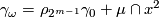$\gamma_\omega = \rho_{2^{m-1}}\gamma_0 + \mu\cap x^2$$\gamma_\omega = \rho_{2^{m-1}}\gamma_0 + \mu\cap x^2$ and $\Gamma_\omega = \langle x,\gamma_0 \rangle - \langle x^3,\mu \rangle$$\Gamma_\omega = \langle x,\gamma_0 \rangle - \langle x^3,\mu \rangle$. 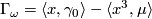Applying this to $(R_3)$$(R_3)$--$(R_5)$$(R_5)$ again, one can see by straightforward checking that $(R_3)$$(R_3)$ and $(R_4)$$(R_4)$ are tautologically true, while $(R_5)$$(R_5)$ turns into

• ($\bar R_5$$\bar R_5$) $\langle x,\gamma\rangle=\langle x^3,\mu\rangle$$\langle x,\gamma\rangle=\langle x^3,\mu\rangle$ for any $x\in H^2(G,2;\,\Zz/2)$$x\in H^2(G,2;\,\Zz/2)$,

using $\gamma$$\gamma$ as abbreviation for $\gamma_0$$\gamma_0$.

Now the relation $(R_1)$$(R_1)$ immediately follows from $(\bar R_5)$$(\bar R_5)$, while $(R_2)$$(R_2)$ can be combined with $(\bar R_5)$$(\bar R_5)$ in the form

• ($R_s$$R_s$) $\langle x,\gamma \rangle = \langle x^3,\mu \rangle$$\langle x,\gamma \rangle = \langle x^3,\mu \rangle$ for any $x\in H^2(G,2;\,\Zz/6)$$x\in H^2(G,2;\,\Zz/6)$.

Hence, for the spin case we have the complete set of invariants $(G,\Delta,\mu,\gamma)$$(G,\Delta,\mu,\gamma)$ with the only relation $(R_s)$$(R_s)$, which gives (for smooth category) the main result of [Zhubr1975].

2.11 The torsion-free case

It is convenient here to represent the additive homology information about some $M\in\mathcal{M}_6^0$$M\in\mathcal{M}_6^0$ by its cohomology group $H=H^2(M)$$H=H^2(M)$, and interpret our previous group $G$$G$ as $\Hom(H,\Zz)$$\Hom(H,\Zz)$. Likewise, the elements of $H_6(G,2)$$H_6(G,2)$ can be considered as symmetric trilinear forms (or cubic forms) on $H$$H$. We thus have the following set of invariants:

• $(H,\ w{\in}H/2H,\ p{:}H{\to}\Zz,\ \Delta{:}H{\to}\Zz/2,\ \mu{:}H^3{\to}\Zz,\ \Gamma_\omega{\in}\Zz,\ \gamma_\omega{:}H{\to}\Zz)$$(H,\ w{\in}H/2H,\ p{:}H{\to}\Zz,\ \Delta{:}H{\to}\Zz/2,\ \mu{:}H^3{\to}\Zz,\ \Gamma_\omega{\in}\Zz,\ \gamma_\omega{:}H{\to}\Zz)$

(for any $\omega\in H$$\omega\in H$ with $\rho_2\omega=w$$\rho_2\omega=w$). We rewrite $(R_1),(R_2)$$(R_1),(R_2)$ in the form:

• $(R_1')$$(R_1')$ $\mu(x,y,x+y+\omega)\equiv0{\mod2}\quad$$\mu(x,y,x+y+\omega)\equiv0{\mod2}\quad$ for any $x,y\in H$$x,y\in H$,
• $(R_2')$$(R_2')$ $p(x)\equiv\mu(x,x,x){\mod3}\quad$$p(x)\equiv\mu(x,x,x){\mod3}\quad$ for any $x\in H$$x\in H$.

Next consider the relations $(R_3)$$(R_3)$ and $(R_4)$$(R_4)$. We can now ``solve´´ them for $\gamma_\omega$$\gamma_\omega$ and $\Gamma_\omega$$\Gamma_\omega$:

• $(R_3')$$(R_3')$ $\displaystyle\gamma_\omega(x)=\frac{p(x)+\mu(\omega,\omega,x)}{4}$$\displaystyle\gamma_\omega(x)=\frac{p(x)+\mu(\omega,\omega,x)}{4}$,
• $(R_4')$$(R_4')$ $\displaystyle\Gamma_\omega=\frac{2\gamma_\omega(\omega) - \mu(\omega,\omega,\omega)}{4}=\frac{p(\omega) - \mu(\omega,\omega,\omega)}{8}$$\displaystyle\Gamma_\omega=\frac{2\gamma_\omega(\omega) - \mu(\omega,\omega,\omega)}{4}=\frac{p(\omega) - \mu(\omega,\omega,\omega)}{8}$.

This shows that $\Gamma$$\Gamma$ and $\gamma$$\gamma$ are expressible in terms of ``classical´´ invariants and should be dropped.

It only remains to consider the last relation $(R_5)$$(R_5)$. We denote by $K$$K$ some (arbitrary) element of $G$$G$ with $\rho_2K=\Delta$$\rho_2K=\Delta$. In view of the above equalities, relation $(R_5)$$(R_5)$ can now be written in the form

• $(R_5')$$(R_5')$ $\displaystyle\frac{p(\omega) - \mu(\omega,\omega,\omega)}{8}\equiv K(\omega) \mod2$$\displaystyle\frac{p(\omega) - \mu(\omega,\omega,\omega)}{8}\equiv K(\omega) \mod2$

or, equivalently,

• $(R_5'')$$(R_5'')$ $(p+8K)(\omega)\equiv\mu(\omega,\omega,\omega)\mod16$$(p+8K)(\omega)\equiv\mu(\omega,\omega,\omega)\mod16$.

Now, quite similar to the spin case above, it is an easy exercise to see that $(R_1')$$(R_1')$ follows from $(R_5'')$$(R_5'')$, while $(R_2')$$(R_2')$ and $(R_5'')$$(R_5'')$ together are equivalent to

• $(R_f)$$(R_f)$ $(p+24K)(\omega)\equiv\mu(\omega,\omega,\omega)\mod48$$(p+24K)(\omega)\equiv\mu(\omega,\omega,\omega)\mod48$.

We have, therefore, the complete set of invariants $(H,w,p,\Delta,\mu)$$(H,w,p,\Delta,\mu)$ satisfying the only relation $(R_f)$$(R_f)$, which gives Theorem 1 of [Jupp1973]; restricting to $\Cat=\Diff$$\Cat=\Diff$ and $w=0$$w=0$, we obtain Theorem 5 of [Wall1966].

Remark 2.5.

1. Relations $(R_3')$$(R_3')$ and $(R_4')$$(R_4')$ can be written, for a manifold $M$$M$, in the form $\gamma_\omega=\frac14D(p_1(M)+\omega^2)$$\gamma_\omega=\frac14D(p_1(M)+\omega^2)$ and $\Gamma_\omega=\frac18\langle p_1(M)\omega-\omega^3,[M]\rangle$$\Gamma_\omega=\frac18\langle p_1(M)\omega-\omega^3,[M]\rangle$, respectively. The fact that $p_1(M)+\omega^2$$p_1(M)+\omega^2$ is divisible by 4 is due to Wu formulas ``modulo 2´´ (for Stiefel-Whitney classes) and ``modulo 4´´ (for Pontryagin classes). The divisibility of the second expression by 8 can be explained as follows: there exists a 4-submanifold $N\subset M$$N\subset M$ dual to the cohomology class $\omega$$\omega$; any such $N$$N$ is spin, and its first Pontryagin class ($=3$$=3$~times its signature) is equal to $(p_1(M)-\omega^2)|_N$$(p_1(M)-\omega^2)|_N$.
2. The fact that relation $(R_1)/(R_1')$$(R_1)/(R_1')$ is excessive in the spin case went unnoticed in both [Wall1966] and [Zhubr1975].
3. Relation $(R_f)$$(R_f)$ in the case of Wall, i.e. for $\omega=2x$$\omega=2x$ and $K$$K$ even, simplifies to
   • $(R_w)$$(R_w)$ $p(x)\equiv4\mu(x,x,x)\mod24$$p(x)\equiv4\mu(x,x,x)\mod24$.
4. The proof of $(R_w)$$(R_w)$ given by Wall relies on construction of 6-manifolds of the type considered by surgery on $S^6$$S^6$ along framed 3-dimensional links, and on relations between the invariants of such links (studied by Haefliger) and the invariants of the resulting manifolds (i.e. $p$$p$ and $\mu$$\mu$). On the other hand, the proof of the more complicated relation $(R_f)$$(R_f)$ in [Jupp1973] is based on integrality theorem for $\hat A$$\hat A$-genus. In fact, for smooth case this follows immediately; regretfully, the argument Jupp gives to extend this to $\Top$$\Top$ category is incorrect, as it uses the erroneous homotopy classification theorem of [Wall1966] (see [Zhubr2000, Subsection 5.14]).

3 Examples and constructions

• The $r$$r$-fold connected sum $\sharp_r S^3\times S^3$$\sharp_r S^3\times S^3$ gives the only element of $\mathcal{M}^{2r}_6(0)$$\mathcal{M}^{2r}_6(0)$.
• The $r$$r$-fold connected sum $M=\sharp_r S^2\times S^4$$M=\sharp_r S^2\times S^4$ gives the ``primary´´ element of $\mathcal{M}^0_6(\mathbb{Z}^r,0)$$\mathcal{M}^0_6(\mathbb{Z}^r,0)$ --- a manifold with $I(M)=(p,\mu)=0$$I(M)=(p,\mu)=0$.
• In the same way, the non-trivial $SO(5)$$SO(5)$-bundle $S^2\tilde\times S^4$$S^2\tilde\times S^4$ is the ``primary´´ element of $\mathcal{M}^0_6(\mathbb{Z},1)$$\mathcal{M}^0_6(\mathbb{Z},1)$.
• The two examples above can be easily generalized: let $w:\mathbb{Z}^r\to\mathbb{Z}/2$$w:\mathbb{Z}^r\to\mathbb{Z}/2$ be arbitrary homomorphism. Let $M$$M$ be the connected sum $\sharp M_i$$\sharp M_i$, where each $M_i$$M_i$ is either $S^2\times S^4$$S^2\times S^4$ or $S^2\tilde\times S^4$$S^2\tilde\times S^4$, depending on the value $w$$w$ takes at the $i$$i$-th basis vector of $\mathbb{Z}^r$$\mathbb{Z}^r$. Then we have $M\in\mathcal{M}^0_6(\mathbb{Z}^r,w)$$M\in\mathcal{M}^0_6(\mathbb{Z}^r,w)$ and $I(M)=0$$I(M)=0$.
• Surgery lets us extend the above construction to arbitrary $(G,w)\in\Hom(\mathcal{A},\mathbb{Z}/2)$$(G,w)\in\Hom(\mathcal{A},\mathbb{Z}/2)$. Take any epimorphism $f:\mathbb{Z}^r\to G$$f:\mathbb{Z}^r\to G$ and build a manifold $M_0\in\mathcal{M}^0_6(\mathbb{Z}^r,w\circ f)$$M_0\in\mathcal{M}^0_6(\mathbb{Z}^r,w\circ f)$ as above. Now represent a free basis of $\Ker f$$\Ker f$ by embedded spheres $S^2\to M_0$$S^2\to M_0$ and do surgery on $M_0$$M_0$ along these spheres. As may be checked, the result is a manifold $M\in\mathcal{M}^0_6(G,w)$$M\in\mathcal{M}^0_6(G,w)$ with $I(M)=0$$I(M)=0$ (therefore, uniquely defined).
• The $SO(3)$$SO(3)$-bundles $M_\beta=S^4\tilde\times_\beta S^2$$M_\beta=S^4\tilde\times_\beta S^2$, with $\beta\in\pi_3(SO(3))=\mathbb{Z}$$\beta\in\pi_3(SO(3))=\mathbb{Z}$, give us manifolds in $\mathcal{M}^0_6(\mathbb{Z},0)$$\mathcal{M}^0_6(\mathbb{Z},0)$ with $I(M_\beta)=(4\beta,\beta)$$I(M_\beta)=(4\beta,\beta)$; in particular, $M_1=\mathbb{C} P^3$$M_1=\mathbb{C} P^3$.
• Complex algebraic geometry makes (potentially) a very powerful source of examples. In particular, any regular complete intersection $M_d$$M_d$ of complex dimension 3 represents an element of $\mathcal{M}^r_6(\mathbb{Z},w)$$\mathcal{M}^r_6(\mathbb{Z},w)$, where $r,w$$r,w$ and $I(M_d)=(p,\mu)$$I(M_d)=(p,\mu)$ can be directly calculated from the multidegree $d=(d_1,\ldots,d_m)$$d=(d_1,\ldots,d_m)$ (see ``Complete intersections´´). In the easiest case --- when $M_d\subset\mathbb{C} P^4$$M_d\subset\mathbb{C} P^4$ is a non-singular hypersurface of degree $d$$d$ --- we have $M_d\in\mathcal{M}^r_6(\mathbb{Z},\rho_2(d-1))$$M_d\in\mathcal{M}^r_6(\mathbb{Z},\rho_2(d-1))$, $I(M_d)=(d(5-d^2),d)$$I(M_d)=(d(5-d^2),d)$, and $r=d^4+\ldots$$r=d^4+\ldots$ (a polynome in $d$$d$ of degree 4).

4 References

• [Jupp1973] P. E. Jupp, Classification of certain $6$$6$-manifolds, Proc. Cambridge Philos. Soc. 73 (1973), 293–300. MR0314074 (47 #2626) Zbl 0249.57005
• [Kirby&Siebenmann1977] R. C. Kirby and L. C. Siebenmann, Foundational essays on topological manifolds, smoothings, and triangulations, Princeton University Press, Princeton, N.J., 1977. MR0645390 (58 #31082) Zbl 0361.57004
• [Okonek&Van de Ven1995] C. Okonek and A. Van de Ven, Cubic forms and complex $3$$3$-folds, Enseign. Math. (2) 41 (1995), no.3-4, 297–333. MR1365849 (97b:32035) Zbl 0869.14018
• [Smale1962] S. Smale, On the structure of $5$$5$-manifolds, Ann. of Math. (2) 75 (1962), 38–46. MR0141133 (25 #4544) Zbl 0101.16103
• [Thomas1956] E. Thomas, A generalization of the Pontrjagin square cohomology operation, Proc. Nat. Acad. Sci. U.S.A. 42 (1956), 266–269. MR0079254 (18,57b) Zbl 0071.16302
• [Wall1966] C. T. C. Wall, Classification problems in differential topology. V. On certain $6$$6$-manifolds, Invent. Math. 1 (1966), 355-374; corrigendum, ibid 2 (1966), 306. MR0215313 (35 #6154) Zbl 0149.20601
• [Zhubr1973] A. V. Zhubr, A decomposition theorem for simply connected 6-manifolds, LOMI seminar notes 36 (1973), 40–49. (Russian)
• [Zhubr1975] A. V. Zhubr, Classification of simply connected six-dimensional spinor manifolds, (English) Math. USSR, Izv. 9 (1975), (1976), 793–812 . Zbl 0337.57004
• [Zhubr2000] A. V. Zhubr, Closed simply connected six-dimensional manifolds: proofs of classification theorems, Algebra i Analiz 12 (2000), no.4, 126–230. MR1793619 (2001j:57041)